An analysis of the Longbeach Animal Shelter dataset

tidy tuesday
r
linear regression
data analysis
Author

Liam Cottrell

Published

March 3, 2025

Introduction

This week’s #TidyTuesday is an exploration of data from an animal shelter in California. I spent an unreasonable amount of time learning how to build a waffle plot.

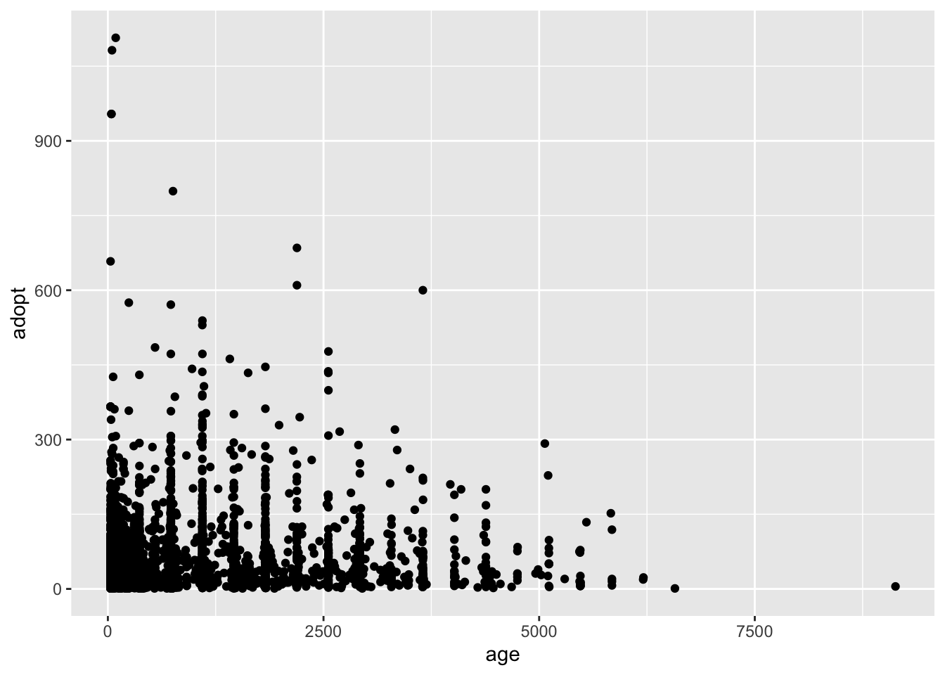
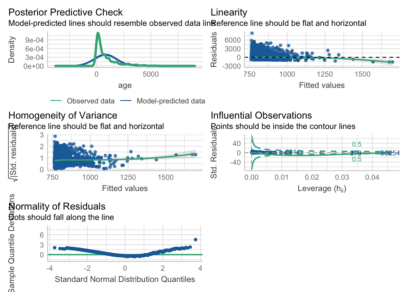
I have also been learning about linear regression so have made a very shoddy attempt to build a model! It doesn’t work because the data is not normally distributed…so at least I know that now 🥲

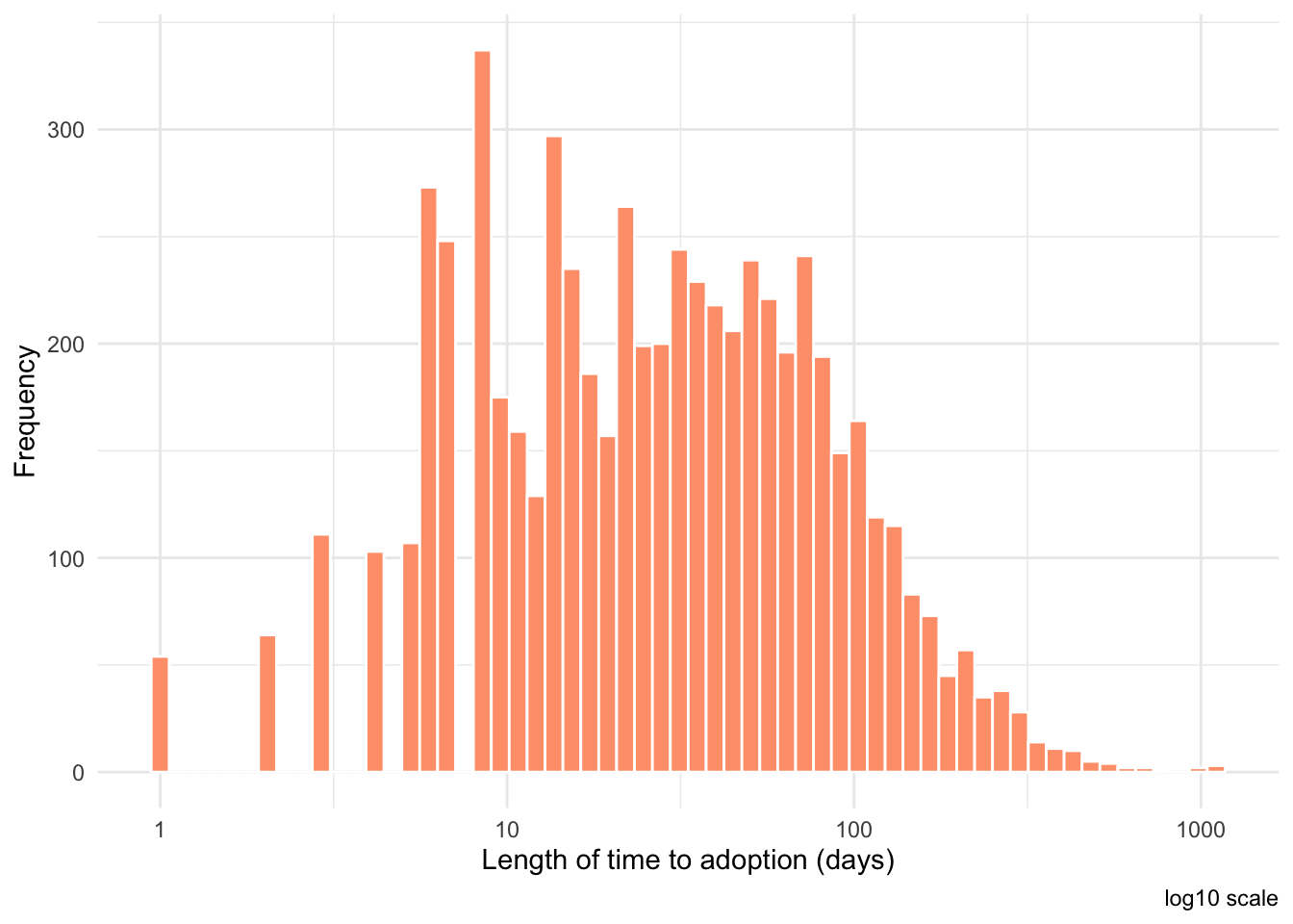
Q1. How long does it take an animal to be adopted from a shelter in California?

# figure out adoption times, remove NAs and 0 days
adoption <- longbeach %>%
  select(intake_date, outcome_date, outcome_type) %>%
  filter(outcome_type == 'adoption') %>%
  mutate(adoption_time = as.numeric(outcome_date -intake_date, na.rm=TRUE)) %>%
  filter(!is.na(adoption_time)) %>%
  filter(adoption_time > 0) %>%
  arrange(-adoption_time)

head(adoption)
# A tibble: 6 × 4
  intake_date outcome_date outcome_type adoption_time
  <date>      <date>       <chr>                <dbl>
1 2019-06-29  2022-07-10   adoption              1107
2 2019-09-11  2022-09-07   adoption              1092
3 2019-07-24  2022-07-10   adoption              1082
4 2019-11-15  2022-06-26   adoption               954
5 2019-11-15  2022-06-26   adoption               954
6 2018-12-19  2021-02-25   adoption               799

Exploratory Data Analysis

# adoption times descriptive statistics
time <- adoption$adoption_time
summary(time)
   Min. 1st Qu.  Median    Mean 3rd Qu.    Max. 
   1.00   11.00   27.00   48.61   62.00 1107.00 
# histogram of adoption times
ggplot(adoption, aes(x = adoption_time)) +
  geom_histogram(bins = 60, fill = "#FFA07A", color = "white") +
  scale_x_log10() +
  labs(x = "Length of time to adoption (days)", 
       y = "Frequency",
       caption = "log10 scale") +
  theme_minimal()

Hypothesis test

The null hypothesis is \(H_0: \mu = 48.61\).

# hypothesis test
t.test(time, mu = 48.61, alternative = "two.sided")

    One Sample t-test

data:  time
t = -0.0028233, df = 6245, p-value = 0.9977
alternative hypothesis: true mean is not equal to 48.61
95 percent confidence interval:
 46.93340 50.28178
sample estimates:
mean of x 
 48.60759 

The p-value is 0.998 so we fail to reject the null hypothesis. Based on the data, we are 95% confident that the average time taken for an animal to be adopted from a shelter in California is between 46.9 and 50.3 days.

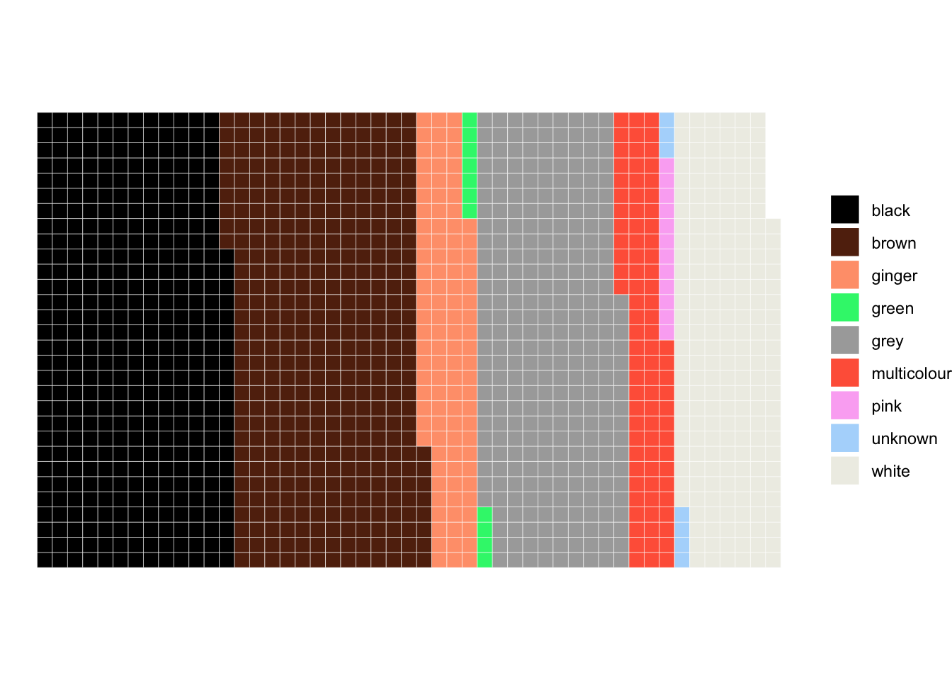
Q2. Which animal colours are most common at the shelter?

# analyse colour
colour_animal <- longbeach %>%
  count(primary_color, name = "Frequency") %>%
  filter(Frequency > 10) %>%
  arrange(-Frequency)
colour_animal
# A tibble: 49 × 2
   primary_color Frequency
   <chr>             <int>
 1 black              7540
 2 gray               3916
 3 white              3651
 4 brown              3531
 5 brown  tabby       2242
 6 tan                1393
 7 gray tabby         1189
 8 orange tabby        904
 9 calico              520
10 orange              515
# ℹ 39 more rows

Consolidate colours into simplified categories

# very unscientific grouping - for learning purposes only
colour_animal <- colour_animal %>%
  mutate(primary_color = case_when(
    primary_color %in% c('orange tabby', 'apricot', 'blonde', 'fawn', 'flame point', 'gold', 'orange', 'red', 'red merle', 'yellow', 'yellow brindle') ~ 'ginger',
    primary_color %in% c('black', 'black smoke', 'black tabby') ~ 'black',
    primary_color %in% c('grey lilac', 'silver tabby','gray tabby', 'blue', 'blue brindle', 'blue merle', 'blue point', 'gray', 'seal', 'seal point', 'silver') ~ 'grey',
    primary_color %in% c('brown', 'brown tabby', 'brown merle', 'brown brindle', 'buff', 'chocolate', 'chocolate point', 'tan', 'brown tiger', 'brown  merle', 'brown  tabby') ~ 'brown',
    primary_color %in% c('cream tabby', 'cream', 'snowshoe', 'white') ~ 'white',
    primary_color %in% c('lynx point', 'lilac point', 'point', 'tricolor', 'lilac lynx point', 'calico', 'calico dilute', 'calico tabby', 'calico point', 'torbi', 'tortie', 'tortie dilute') ~ 'multicolour',
    TRUE ~ primary_color
  )) %>%
  arrange(primary_color)
# waffle plot of colours
ggplot(colour_animal, aes(fill=primary_color, values=Frequency/20)) +
  geom_waffle(color = "white", size = 0.1, n_rows = 30) +
  theme_void() +
  coord_fixed(ratio = 1) +
  scale_fill_manual(values = c("#000000", "#622a0f", "#FFA07A", "#2df47a", "#a9a9a9", "#FF6347", "#fbb1f3","#b1d9fb","#eeeee6" )) +
  theme(legend.title = element_blank()) 

Q3. Is there a relationship between animal age and length of time to adopt?

animal_stats <- longbeach %>%
  select(intake_date, outcome_date, outcome_type, dob) %>%
  filter(outcome_type == 'adoption') %>%
  mutate(adoption_time = as.numeric(outcome_date -intake_date, na.rm=TRUE)) %>%
  mutate(intake_age = as.numeric(intake_date - dob, na.rm=TRUE)) %>%
  filter(!is.na(adoption_time)) %>%
  filter(!is.na(intake_age)) %>%
  filter(adoption_time > 0) %>%
  filter(intake_age > 30) %>%
  arrange(intake_age)

head(animal_stats)
# A tibble: 6 × 6
  intake_date outcome_date outcome_type dob        adoption_time intake_age
  <date>      <date>       <chr>        <date>             <dbl>      <dbl>
1 2022-08-24  2022-09-17   adoption     2022-07-24            24         31
2 2023-04-30  2023-10-25   adoption     2023-03-30           178         31
3 2022-09-22  2022-12-23   adoption     2022-08-22            92         31
4 2023-09-19  2024-01-17   adoption     2023-08-19           120         31
5 2023-09-19  2024-01-18   adoption     2023-08-19           121         31
6 2023-09-19  2024-01-17   adoption     2023-08-19           120         31
age <- c(animal_stats$intake_age)
adopt <- c(animal_stats$adoption_time)
sum(age > 0)
[1] 5366
sum(adopt > 0)
[1] 5366
with(animal_stats, cor(intake_age, adoption_time))
[1] 0.05643874
#with(animal_stats, cor.test(intake_age, adoption_time))
ggplot(animal_stats, aes(x = age, y = adopt)) +
  geom_point() 

model1 <- lm(age ~ adopt, data=animal_stats)
summary(model1)

Call:
lm(formula = age ~ adopt, data = animal_stats)

Residuals:
    Min      1Q  Median      3Q     Max 
-1629.3  -697.1  -410.8   311.0  8364.1 

Coefficients:
            Estimate Std. Error t value Pr(>|t|)    
(Intercept) 762.6651    16.7708   45.48  < 2e-16 ***
adopt         0.8453     0.2042    4.14 3.52e-05 ***
---
Signif. codes:  0 '***' 0.001 '**' 0.01 '*' 0.05 '.' 0.1 ' ' 1

Residual standard error: 1017 on 5364 degrees of freedom
Multiple R-squared:  0.003185,  Adjusted R-squared:  0.002999 
F-statistic: 17.14 on 1 and 5364 DF,  p-value: 3.524e-05
library(performance)
check_model(model1)