Report
Introduction
Being a victim of crime as a child can cause long-lasting trauma, contributing to poor health and education outcomes (Morgan and Zedner, 1992). Children who are victimised also have a higher likelihood of committing violent behaviour or future offending themselves (AuCoin, 2005). Breaking this cycle is a critical challenge for policymakers, law enforcement, and communities.
According to some sources, certain types of crime in Los Angeles are decreasing (Fioresi and Nguyen, 2025). However, between January 2010 and May 2025, there were almost 130,000 recorded victims of crime under the age of 18 (City of Los Angeles, 2025a; 2025b), highlighting the need for intervention.
Research into understanding and predicting crime patterns has a centuries-long history (Wills, 2023). As Jenga, Catal and Kar (2023) explain, crimes are ‘not distributed evenly and uniformly nor are they random’; rather, “hotspots” where criminal activity is more concentrated are often observed. Understanding the different dynamics involved is, therefore, essential when considering crime prevention strategies (Bediroglu and Çolak, 2024).
Problem Definition
This project does not attempt a general model of crime prediction, but focuses on understanding child victimisation risk through applying machine learning to Los Angeles Police Department crime reports from 2010–2025.
Child victimisation is framed as a supervised classification problem; the model uses demographic, spatial, temporal, and situational attributes of reported crimes to predict whether the victim is under 18. The objective is to identify potential risk factors and generate insights that could inform child protection strategies.
Data Exploration and Preparation
First, two publicly-available crime datasets were obtained as CSV files from the US Government data portal and combined. The data were visualised and cleaned through an iterative approach that explored trends and guided feature engineering, consistent with Banyin’s (2019) view that these are concurrent processes.
A summary is shown in Table 1.
| Original features (including: victim demographics, crime type, date/time occurred/reported, location) | 28 |
| Observations (2010-19) | 2,133,202 |
| Observations (2020-25) | 1,004,991 |
| Duplicates removed | 60,175 |
| Final dataset (after cleaning and encoding) | 2,445,380 observations 60 features 1 label (Boolean |
Table 1
Child-only and adult-only subsets were created, explored separately, and compared. Features showing notable differences between children and adults – such as trends in premises where crimes occurred – were scrutinised further. At this stage, the analysis was primarily descriptive and bivariate, whilst the modelling itself is multivariate, aiming to ‘determine which variables influence or cause the outcome’ (Bush 2022).
Considerations
Various factors were accounted for when preparing the data. First, the data were highly imbalanced with only 5% relating to child victims (is_child = 1). This imbalance required attention to ensure that minority class cases were not overlooked.
Several features showed high cardinality with some low-frequency categories. To address this, relevant values were aggregated with categories representing fewer than 1% of cases grouped as “Other/Unknown” (Sangani, 2021).
Finally, some variables were encoded to ensure compatibility with machine learning algorithms – this encompassed one-hot encoding for categorical data (Rojo-Echeburúa, 2024) and cyclical encoding for temporal variables such as month and hour (Pelletier, 2024).
Trends
Temporal
A problem was observed with recording of crime incidents; large spikes are visible at 12pm and the first of the month. As Kaplan (2025) notes, ‘when agencies are unsure of the exact date of a crime, they appear to default to entering the 1st of the month as a placeholder’. Hot-deck (kNN) imputation was applied to reduce the over-representation of 12pm. However, the day_of_month variable was dropped rather than imputed, as it was unlikely to provide meaningful predictive value. Following imputation, two clear daily peaks emerged for child victims: around 8am and 3pm (Figure 1). This likely reflects school travel times, when children are in public and less supervised.
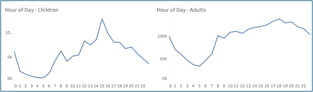
Figure 1
Weekly patterns showed a small Friday peak, especially for children, while weekends saw a sharp decline in child victimisation compared with adults (Figure 2).
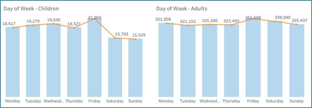
Figure 2
A dip in child victimisation was evident in July, in contrast with broader criminological findings that crime tends to rise in summer (Medina & Solymosi, 2022). In contrast, adult victimisation remained relatively stable across the year (Figure 3).
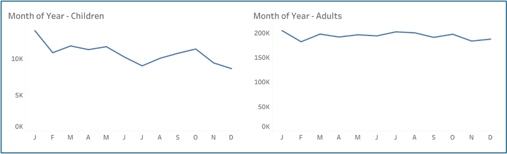
Figure 3
These temporal differences between victimisation of adults and children informed the inclusion of hour, day, and month as features in the model.
Demographic
Across all ages under 18, girls were more frequently victimised than other genders, particularly for teenagers (Figure 4). In adult populations, however, men were more often victims than women.
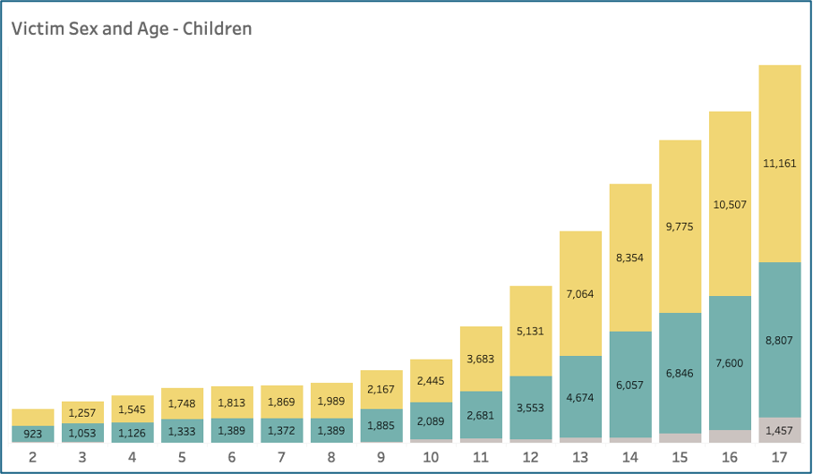
Figure 4
Ethnic disparities were evident. Figure 5 shows how Hispanic/Latin/Mexican and Black children were disproportionately affected, compared to the proportions they represent in Los Angeles’ total population (United States Census Bureau, 2023). For adults, Black adults remained over-represented but Hispanic/Latin/Mexican rates dropped and white adult victimisation increased.
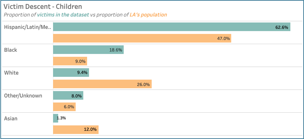
Figure 5
Spatial
Unsurprisingly, crimes at educational premises were more prevalent for children than adults (Figure 6).
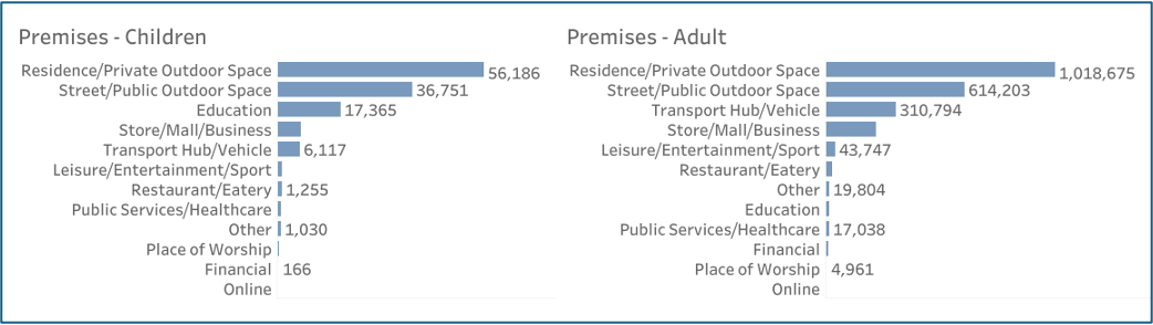
Figure 6
The 77th Street area recorded the highest rates of child victimisation. Differences across ethnic groups largely reflected neighbourhood demographics; for example, West LA reported more white child victims, aligning with the area’s population profile (Statistical Atlas, 2018).
For modelling, categorical area names were used instead of latitude and longitude, which can yield stronger performance (Feifke, 2024).
Situational
Adults were more likely to be victims of theft, whereas children were more frequently victims of assault or violence, with sexual offences ranking third for children compared with fifth for adults (Figure 7).
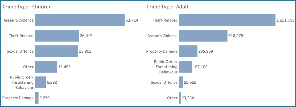
Figure 7
Weapon use also varied: males were more likely than females to be victims of firearms across age groups, while for children the most common categories were bodily force or no/unknown weapon (Figure 8).
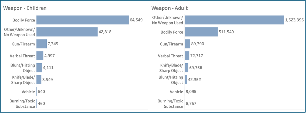
Figure 8
Algorithm Selection
As a classification problem, the task is within scope of several algorithms. Four were selected due to their suitability: k-Nearest Neighbours, Random Forest, Naïve Bayes, and Logistic Regression.
Various metrics (precision, recall, accuracy and ROC AUC) were scrutinised but, given the context of this study, recall was prioritised to guide model selection.
To support robust model comparison, a four-step selection process was adopted. First, initial selection was conducted, based on research. Next, a simple train–test split was used to gauge performance in a prototyping scenario. Cross-validation with RandomizedSearch and Stratified K-Fold was then applied to optimise hyperparameters. Lastly, a final model was trained using the identified parameters.
Stage 1: Initial Selection
K-Nearest Neighbours (KNN) was quickly ruled out, as one-hot encoded features do not provide meaningful distance metrics, and the dataset’s scale would likely result in an inefficient training process (Joby, 2025).
Stage 2: Prototyping
Although Random Forest achieved an ROC-AUC score of 0.84, its recall was the lowest of all models tested (0.28). Whilst its F1 score was also higher, this was driven by precision rather than recall. This suggests that the model would fail to identify a large proportion of child victims, which makes it unsuitable despite its ability to classify well.
Stage 3: RandomizedSearch
Naïve Bayes performed well; in fact, its recall score was higher than Logistic Regression (Figure 9). However, it was ultimately rejected for two reasons:
-
Its assumption of feature independence is unsuitable for this dataset (Chauhan, 2022). For example, there is clearly dependence between
premisesandday; crimes in schools occur substantially more on weekdays than weekends. This is particularly pertinent as explained later – education premises is the most important feature in the model. - Relevant studies have shown that naïve predictive models struggle to capture spatio-temporal crime patterns effectively (Kadar, Maculan & Feuerriegel, 2018).
Stage 4: Final Model
Logistic Regression was used as the final model, as it offered good recall and ROC-AUC once parameters were optimised. SMOTE was applied during training to address the class imbalance, helping the model better detect child cases (Singh, 2025). Importantly, Logistic Regression also provides interpretable coefficients (Payong and Mukherjee, 2025), which supports the achievement of the project’s objective to identify actionable insights, as risk factors for child victimisation can be quantified.
Figure 9 shows the best scores achieved for each of the tested algorithms.
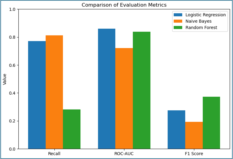
Figure 9
Evaluation
Metrics
Given the safeguarding context of this study, recall was prioritised over other metrics. The aim was to minimise false negatives so that as many cases of child victimisation as possible were captured in the analysis. Whilst the project does not directly identify children at risk, maximising recall ensured that patterns of child victimisation were not overlooked, increasing the likelihood of uncovering meaningful predictors. This necessarily came with a trade-off against precision, but it was judged acceptable in this context.
The final Logistic Regression model achieved recall of 0.77, so successfully identified the majority of children. Precision was low (0.17), reflecting a large number of false positives. Overall accuracy was 0.79, but this metric is less meaningful in the context of class imbalance (Goyal, 2021). The classification report (Figure 10) illustrates the disparity between the two classes, showing much stronger performance for adults than children, but still confirming that recall on is_child = 1 was robust.
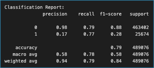
Figure 10
The confusion matrix (Figure 11) further reinforces the findings above. The model correctly classified 19,791 child cases but missed 5,883, while a large number of adults (97,651) were incorrectly predicted as children. This is deemed to be acceptable for the use case, although it is acknowledged that precision is reduced so any insights should be treated with caution.
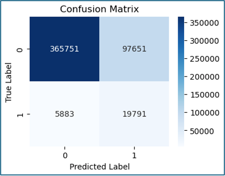
Figure 11
The ROC curve (Figure 12) shows that the model is relatively good at discriminating between the classes, with a ROC-AUC score of 0.86.
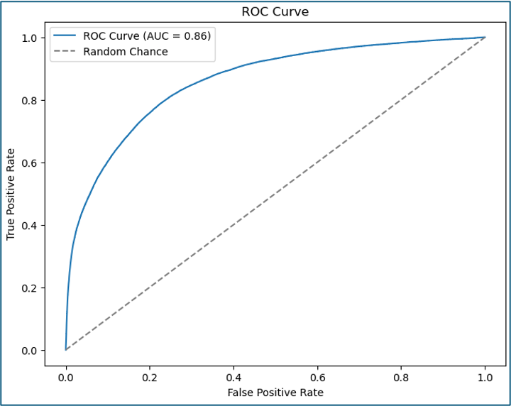
Figure 12
However, it is argued that ROC-AUC may be less reliable in highly imbalanced datasets, so an AUPRC curve was also plotted (Figure 13). The area under the curve (AP = 0.375) further confirms that, although the model achieves moderate recall, this comes at the expense of precision. The model is somewhat better at classifying the minority class than random chance (Rosenberg, 2022), demonstrating its potential for identifying vulnerable children in contexts where missing a positive case is far more costly than creating some false alarms.
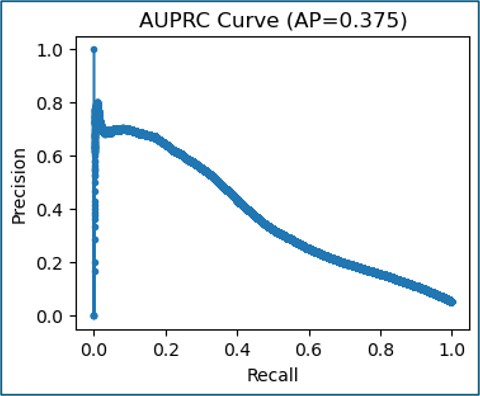
Figure 13
Feature Importance
Examining feature importance through ELI5 helps with interpretation of the model’s results into real-world insights.
Figure 14 shows that crimes in educational premises had the strongest positive association with child victims, which is consistent with the EDA and thereby helps to validate the model. The next two most influential features – crime_other and vict_sex_other_unknown – potentially indicate a problem with noise as they are not interpretable into a useful real-world context.
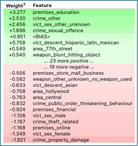
Figure 14
Temporal variables did not appear in the top 20 features, suggesting that although some seasonality was noted during EDA, these patterns were not sufficiently strong to contribute to predictive performance.
Overall, the evaluation suggests that Logistic Regression was an appropriate final choice, delivering recall strong enough to ensure that most child cases were identified and offering interpretable coefficients that provide insight into potential risk factors. At the same time, the high false positive rate and low precision mean that results must be interpreted with caution. The model offers exploratory usage for understanding associations that may inform safeguarding discussions, but is not recommended to be used for decision-making about individual children.
Conclusion
The model in this study can be used cautiously to highlight which factors are most strongly associated with risk of child victimisation and, therefore, where interventions could be targeted.
Excluding the less interpretable “other” categories, the model identified risk related to crimes occurring in educational premises, sexual offences, incidents within the 77th Street area, and victims from Hispanic/Latin/Mexican backgrounds. These features do not necessarily describe a single type of victim or incident; rather, they represent separate conditions under which child victimisation is more likely.
From a practical perspective, such insights could help inform targeted safeguarding strategies. For example, funding could be given to a youth centre in 77th Street, to run outreach programmes for Hispanic youth to offer them safe spaces or structured activities. The model is exploratory and should not be considered a definitive predictive system, but it can provide a useful starting point for exploring how child victimisation in Los Angeles can be addressed and reduced.
Limitations and Scope for Future Work
This study has several limitations that should be acknowledged:
- The dataset records reported crimes rather than convictions, so it reflects reporting behaviour rather than confirmed criminal outcomes.
- Aggregating high-cardinality variables improved robustness but this can also mask important distinctions, which can ‘lose the granularity we need to derive insights’ (Fayard, 2025).
- Methodologically, the project could have been improved by building a fully reproducible pipeline, and through more efficiency (such as exporting Parquet files instead of CSV).
Future work could encompass the following areas for improvement:
- Alternatives resampling methods to SMOTE (e.g. undersampling or ensemble techniques) could be explored.
- The recall/precision balance could potentially be addressed through approaches such as cost-sensitive learning or threshold adjustment (Ibezim, 2023).
-
Additional feature engineering could incorporate interaction terms, e.g.
vict_sex_vs_premisesor more granular age categories, to further capture complex relationships.
Whilst Logistic Regression achieved strong recall, low precision means adults were often misclassified as children, so findings should be treated with caution.
Bibliography
AuCoin, K. (2005) Children and Youth as Victims of Violent Crime. Juristat: Canadian Centre for Justice Statistics. 25 (1), pp. 1-24.
Banyin, N. (2024) Exploratory Data Analysis with Excel [blog]. Medium. 7 February. Available from: https://medium.com/@NanaBanyin/exploratory-data-analysis-with-excel-e2b61471df6b [Accessed 8 July 2025].
Bediroglu, G. and Çolak, H.E (2024) Predicting and analyzing crime – Environmental design relationship via GIS-based machine learning approach. Transactions in GIS. 28 (5), pp. 1377-1399.
Bush, J. (2022) The Difference Between Bivariate & Multivariate Analyses [blog]. Sciencing. 24 March. Available from: https://www.sciencing.com/difference-between-bivariate-multivariate-analyses-8667797/ [Accessed 2 July 2025].
Chauhan, N.S. (2022) Naïve Bayes Algorithm: Everything You Need to Know [blog]. KD Nuggets. 8 April. Available from: https://www.kdnuggets.com/2020/06/naive-bayes-algorithm-everything.html [Accessed 1 August 2025].
City of Los Angeles (2025a) Crime Data from 2010 to 2019, LAPD OpenData (2025 version) [online]. Available from: https://catalog.data.gov/dataset/crime-data-from-2010-to-2019 Accessed 20 June 2025].
City of Los Angeles (2025b) Crime Data from 2020 to Present, LAPD OpenData (25 May 2025 version) [online]. Available from: https://catalog.data.gov/dataset/crime-data-from-2020-to-present [Accessed 20 June 2025].
Fayard, M. (2025) Understanding Cardinality: Challenges and Solutions for Data-Heavy Workflows [tutorial]. DataCamp. 13 January. Available from: https://www.datacamp.com/tutorial/cardinality [Accessed 29 July 2025].
Feifke, B. (2024) Feature Engineering With Latitude and Longitude [blog]. Call Me Ben. 26 March. Available from: https://benfeifke.com/posts/feature-engineering-with-latitude-and-longitude/ [Accessed 2 July 2025].
Fioresi, D. and Nguyen, J. (2025) Los Angeles city leaders tout 20% decrease in homicides; city on pace for lowest numbers in 60 years. CBS News. 9 July. https://www.cbsnews.com/losangeles/news/los-angeles-city-leaders-tout-20-decrease-in-homicides-city-on-pace-for-lowest-numbers-in-60-years/ [Accessed 2 August 2025].
Géron, A. (2025) Hands-On Machine Learning with Scikit-Learn and PyTorch. California: O’Reilly.
Goyal, S. (2021) Evaluation Metrics for Classification Models [blog]. Medium. 20 July. Available from: https://medium.com/analytics-vidhya/evaluation-metrics-for-classification-models-e2f0d8009d69 [Accessed 29 July 2025].
Ibezim, C. (2023) Threshold Dilemma in Machine Learning: Balancing Precision and Recall for Optimal Model Performance [blog]. Medium. 22 December. Available from: https://medium.com/@ibezimchike/threshold-dilemma-in-machine-learning-balancing-precision-and-recall-for-optimal-model-performance-eb3dc01e162e [Accessed 12 August 2025].
Joby, A. (2025) K-Nearest Neighbor (KNN) Algorithm: Use Cases and Tips [blog]. University Edge. 2 July. Available from: https://learn.g2.com/k-nearest-neighbor [Accessed 14 August 2025].
Jenga, K., Catal, C. and Kar, G. (2023) Machine learning in crime prediction. Journal of Ambient Intelligence and Humanized Computing. 14, pp. 2887–2913.
Kadar, C., Maculan, R. and Feuerriegel, S. (2019) Public decision support for low population density areas: An imbalance-aware hyper-ensemble for spatio-temporal crime prediction. Decision Support Systems. 119, pp. 107-117.
Kaplan, J. (2025) Decoding FBI Crime Data. Available from: https://ucrbook.com/ [Accessed 31 July 2025].
Legal Clarity California (2024) California Penal Code 288: Violations, Penalties, and Defenses. Available from: https://legalclarity.org/california-penal-code-288-violations-penalties-and-defenses/ [Accessed 3 August 2025].
Medina, J. and Solymosi, R. (2022) Crime Mapping and Spatial Data Analysis using R [online]. Available from: https://maczokni.github.io/crime_mapping/ [Accessed 23 July 2025].
Morgan, J. and Zedner, L. (1992) Child victims: crime, impact and criminal justice. Oxford: Oxford University Press.
OpenAI (2025a) ChatGPT. ChatGPT response to request for assistance with categorisation of weapon types. Available from: https://chatgpt.com/share/68868c05-32b8-8010-8146-77791b125be0 [Accessed 27 July 2025].
OpenAI (2025b) ChatGPT. ChatGPT Agentic response to query regarding definition of crime type “CRM AGNST CHILD”. Available from: https://chatgpt.com/share/688f2eb5-92b4-8010-ab64-e801bcb39553 [Accessed 3 August 2025].
Payong, A. and Mukherjee, S. (2025) Mastering Logistic Regression with Scikit-Learn: A Complete Guide [tutorial]. Digital Ocean. 20 March. Available from: https://www.digitalocean.com/community/tutorials/logistic-regression-with-scikit-learn [Accessed 12 August 2025].
Pelletier, H. (2024) Cyclical Encoding: An Alternative to One-Hot Encoding for Time Series Features. Towards Data Science. Available from: https://towardsdatascience.com/cyclical-encoding-an-alternative-to-one-hot-encoding-for-time-series-features-4db46248ebba/ [Accessed 2 July 2025].
Rojo-Echeburúa, A. (2024) What Is One Hot Encoding and How to Implement It in Python [tutorial]. DataCamp. 26 June. Available from: https://www.datacamp.com/tutorial/one-hot-encoding-python-tutorial [Accessed 16 July 2025].
Rosenberg, D. (2022) Imbalanced Data? Stop Using ROC-AUC and Use AUPRC Instead. Towards Data Science. Available from: https://towardsdatascience.com/imbalanced-data-stop-using-roc-auc-and-use-auprc-instead-46af4910a494/ [Accessed 20 August 2025].
Sangani, R. (2021) Dealing with features that have high cardinality. Towards Data Science. Available from: https://towardsdatascience.com/dealing-with-features-that-have-high-cardinality-1c9212d7ff1b/ [Accessed 29 July 2025].
Singh, H. (2025) 10 Techniques to Solve Imbalanced Classes in Machine Learning [blog]. Analytics Vidhya. 1 May. Available from: https://www.analyticsvidhya.com/blog/2020/07/10-techniques-to-deal-with-class-imbalance-in-machine-learning/ [Accessed 8 July 2025].
Statistical Atlas (2018) Race and Ethnicity in West Los Angeles, Los Angeles, California (Neighborhood). Available from https://statisticalatlas.com/neighborhood/California/Los-Angeles/West-Los-Angeles/Race-and-Ethnicity [Accessed 8 July 2025].
UK Government (2020) Ethnicity data: how similar or different are aggregated ethnic groups?. Available from: https://www.gov.uk/government/publications/ethnicity-data-how-similar-or-different-are-aggregated-ethnic-groups/ [Accessed 16 July 2025].
United States Census Bureau (2023) Los Angeles city, California. Available from: https://data.census.gov/profile/Los_Angeles_city,_California?g=160XX00US0644000 [Accessed 17 June 2025].
Wills, M. (2023) The History of Precrime. JSTOR Daily [online]. Available from: https://daily.jstor.org/the-history-of-precrime/ [Accessed 2 July 2025].